User Manual
This user manual is meant to support you in using the Riverplume Workflow. It contains information on how to get started with the tool and How-To’s for typical applications. In addition, there are details on the implementation and background information regarding the data and algorithms used in the workflow. You can navigate the user manual through the sidebar.
Software and Resources
Additional Resources
In addition to this documentation, we offer the following resources to support users and developers who work with the River Plume Workflow:
detailed READMEs in all software repositories related to the River Plume Workflow
Getting started
In this chapter, we will guide you through your first steps with the River Plume Workflow. We’ll use the workflow to find the Elbe river plume in the North Sea during the 2013 flood.
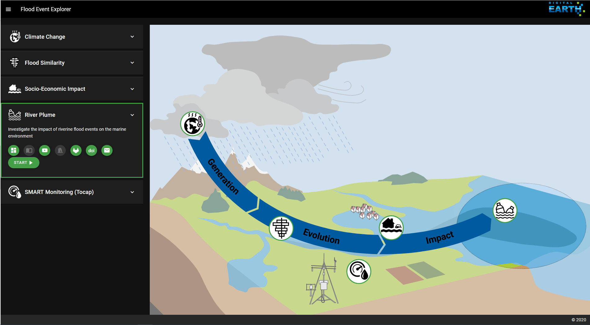
Fig. 2 Landing page of the Digital Earth Flood Event Explorer (FEE)
You can start working with the River Plume Workflow either by installing and running it locally on your machine, as described in section Installation, or you can find the Workflow through the Digital Earth Flood Event Explorer (FEE).
On the Flood Event Explorer (FEE) home page (Fig. 2) choose the River Plume menu. The green buttons in the menu offer additional resources, such as links to a tutorial video, the gitlab repository and this documentation.
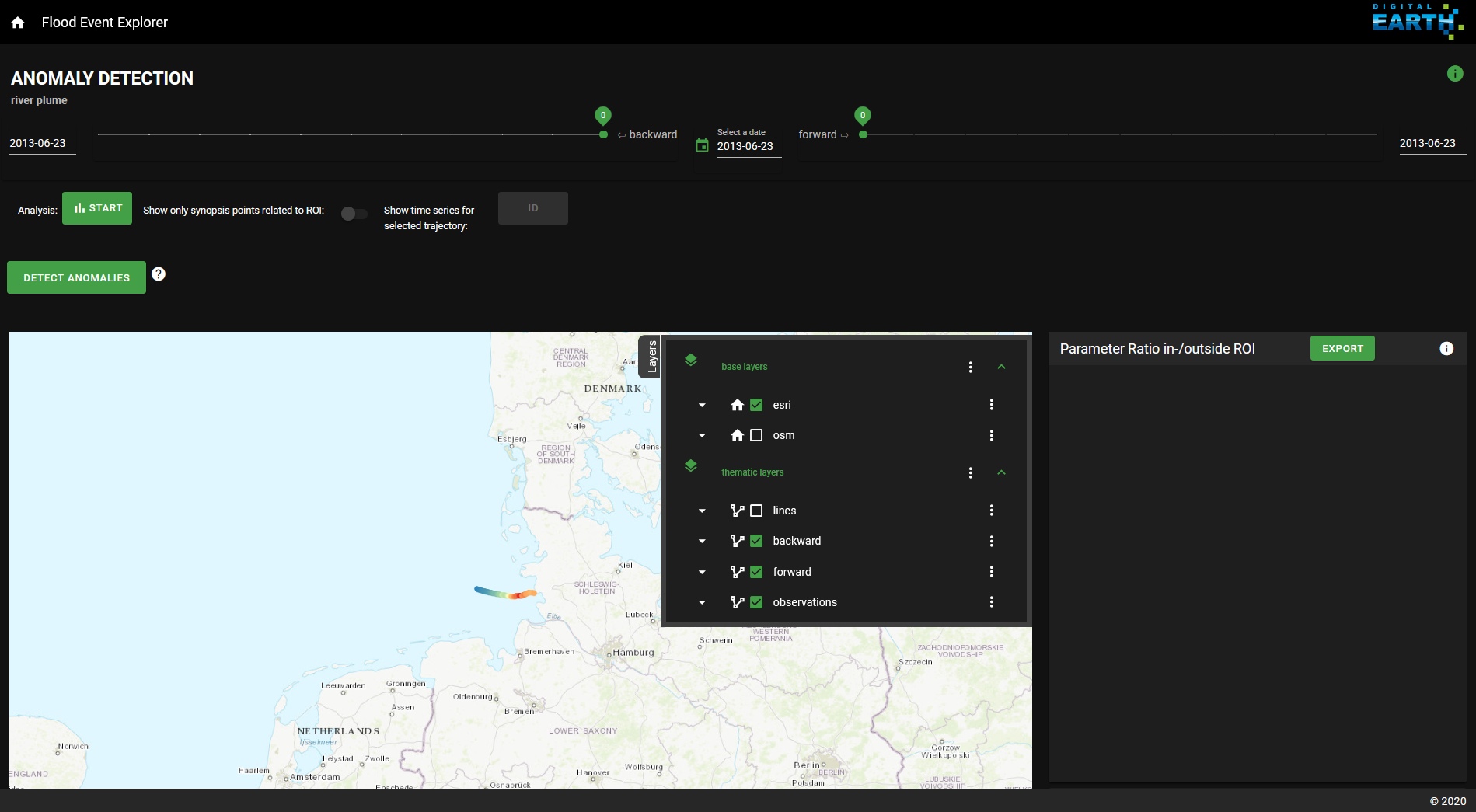
Fig. 3 Landing page of the Riverplume Workflow
The start-button takes you to the River Plume Workflow (Fig. 3). Once there, you can always return to the FEE landing page through the home button on the top left of the River Plume Workflow page. On the top right, you’ll find an info-button with the data source attributions.
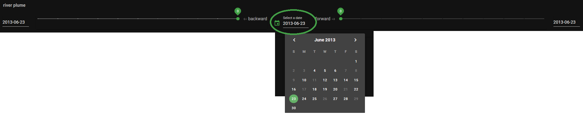
Fig. 4 The calendar menu
We’ll start our search for the Elbe river plume by loading data from FerryBox measurements into the interactive map. For this, click on the date in the upper middle of the page and select a date in the calendar tool (Fig. 4). The observational data belonging to that date are loaded automatically. Days, where no FerryBox transects are available, are greyed out. For our example, we’ll stay with the pre-selected 2013-06-23.
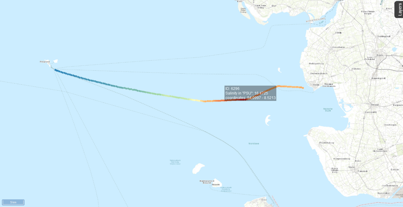
Fig. 5 The selected FerryBox data in the interactive map
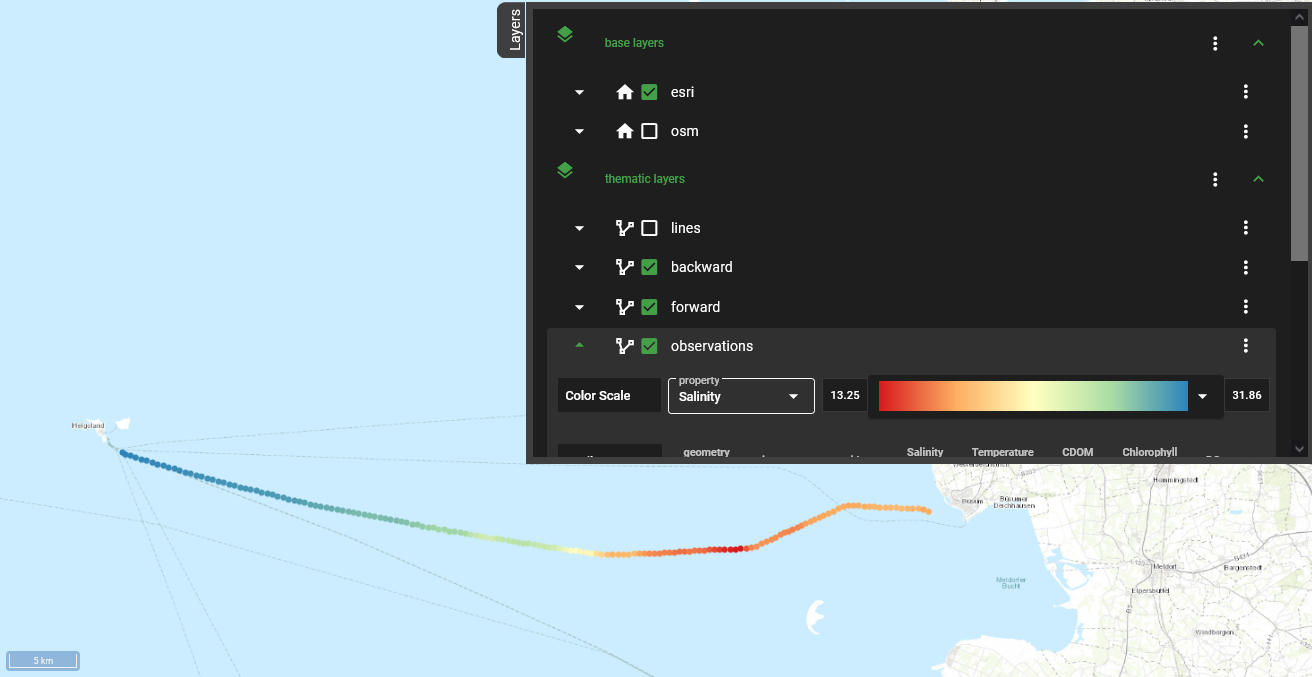
Fig. 6 The layers menu in the interactive map
Now that we chose a date, the Ferrybox measurements are displayed in the interactive map (Fig. 5). Details of a single measurement are displayed when mousing over the respective point on the FerryBox transect. Clicking on the Layers button in the top right corner, opens the Layers menu (Fig. 6). It contains options for displaying the different layers of data. The settings for the FerryBox data can be found under observations. Here, you can select from the list of properties, i.e. observed parameters, and adjust the color scale to your preferences.
In the next step, we use synopsis model data to help us find a region of interest for our presumed Elbe river plume. Using the sliders left and right of the calendar tool (Fig. 4), you can load the matching model trajectories up to 10 days before and after the chosen date. Please note, that model data only is generated for specific events of interest and is not available for every day with FerryBox measurements. A list of events with existing model data can be found in Methods.
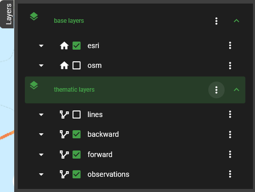
Fig. 7 The Layers menu
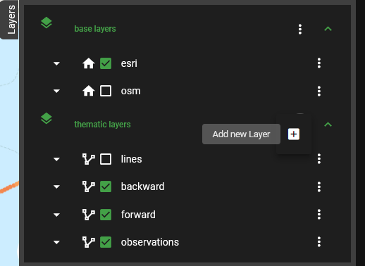
Fig. 8 Add a new layer to the map
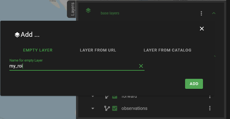
Fig. 9 Name your custom map layer
Now it is time to take a closer look at the data we loaded. Since we are
looking for the Elbe river plume in the FerryBox observations, we are
looking for an anomaly in terms of salinity and chlorophyll. Since the
river plume consists of freshwater, the salinity in the river plume
should be lower than in the surrounding waters. We use chlorophyll-a as
a proxy for biological activity, meaning that a high chlorophyll value
indicates that the water at the point of measurement is richer in
nutrients than its surroundings. We check the FerryBox observations for
anomalies that fit theses criteria by switching between parameters in
the Layers menu (Fig. 7), under observations.
Once we identify a region of interest (ROI), we use the interactive map to mark it for further investigations. For this, we use the Layers menu again and add a new layer to the map by clicking on the three dots next to thematic layers (Fig. 7) and then on the plus sign (Fig. 8). In the pop-up menu, name your new layer and click on the Add button (Fig. 9). We named our layer my_roi.
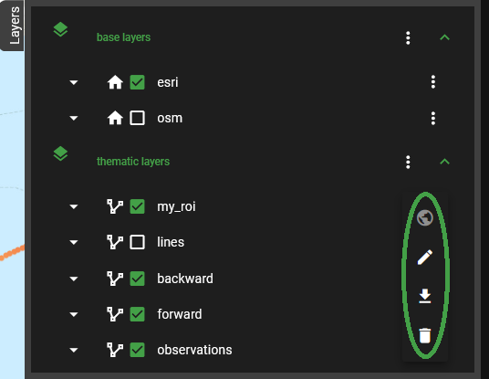
Fig. 10 The options menu for our custom layer
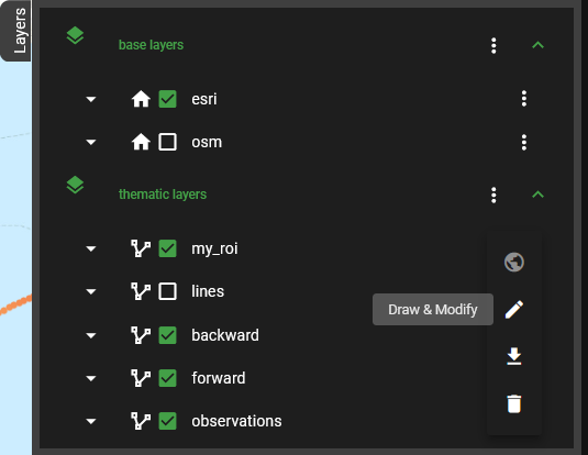
Fig. 11 The Draw & Modify option for custom layers
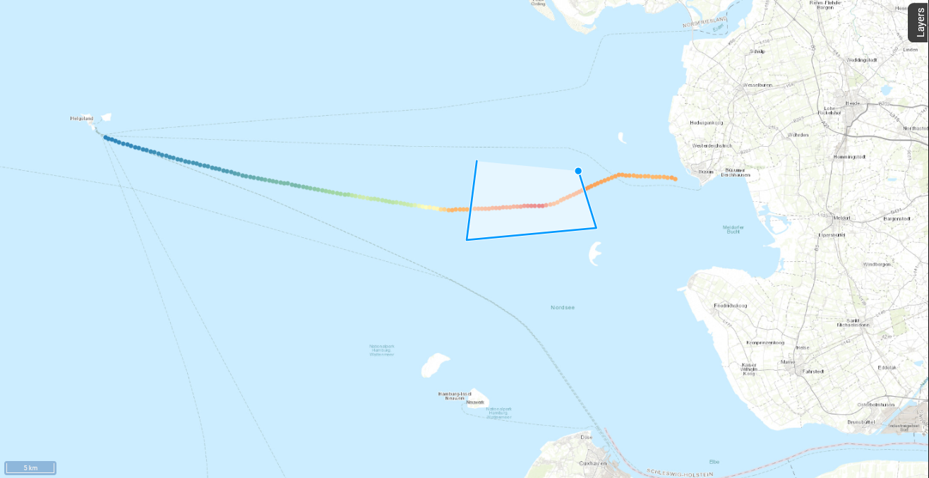
Fig. 12 Using Draw & Modify to mark a region of interest in the map
The new layer now shows up in the list of thematic layers. Clicking on
the three dots next to my_roi opens its options menu
(Fig. 10). We
now select the Draw & Modify option
(Fig. 11). It
allows us to mark our region of interest on the interactive map. Just
click on the map where you want the corners of your region to lie and
close the area by clicking on your first point again
(Fig. 12). By
selecting the Draw & Modify tool again, you stop this mode. The layer
my_roi now contains all points of the Ferrybox transect that fall into
the selected area.
Now that we marked our region of interest, it is time to check if the area shows any signs of containing the river plume we are looking for. In a first step, we activate the toggle switch titled “Show only synopsis points related to ROI” above the map. This way, we can take a closer look at the origin of the data points we selected and check if their modelled trajectories match our expectation. In our case, the selected water bodies actually crossed the Elbe estuary in the last 10 days (see Fig. 13).
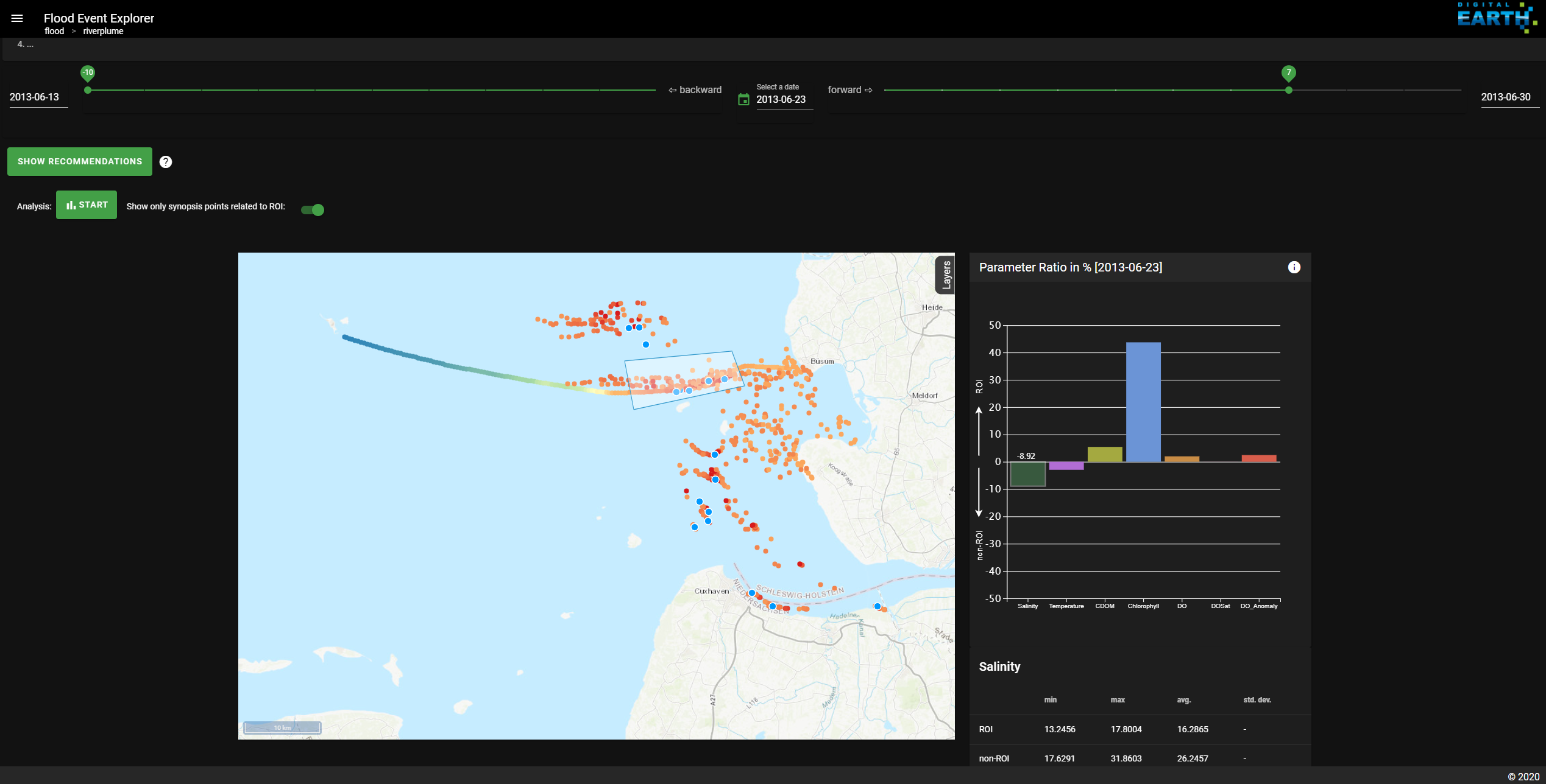
Fig. 13 There is an option to only display the trajectories related to measurments in the ROI .
In a second step, we take a closer look at the water composition in our ROI compared to the other data measured during this FerryBox campaign. The analysis is started through the “Start” button above the map. The result is an interactive bar plot that compares the water composition inside and outside our region of interest based on the FerryBox measurements (see Fig. 14). The chart shows the parameter ratio between measurements inside and outside the ROI in percent. By clicking on one of the bars, details on the value distribution for one parameter are displayed in a table below the chart.
Here, the comparatively lower salinity together with higher chlorophyll-a values point to a fluvial origin of the water bodies in our region of interest.
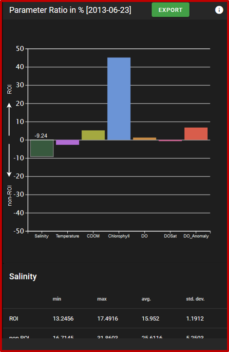
Fig. 14 A bar chart shows the results of the composition analysis.
In our example, the water bodies in our region of interest seem to originate from the Elbe estuary and show temperature and salinity measurements that indicate the presence of fluvial water. Both findings togther are a strong indicator that our selected region of interest indeed contains the Elbe river plume. By clicking the “Export” button in the analysis plot, you can download the FerryBox data annotated with the information whether each measurement lies inside or outside your specified region of interest.
To read more about the advanced applications of the Riverplume Workflow, please check out the How To section.
How-to
This section contains instructions on how to use the Riverplume Workflow to solve commonly encountered tasks.
Task 1: Find riverine extreme events in the FerryBox data
Task 2: Narrow down the river plume candidates
Task 3: Investigate a specific extreme event
Task 4: Generate new datasets for the Riverplume Workflow
Task 1: Find riverine extreme events in the FerryBox data
Coming Soon
Task 2: Narrow down the river plume candidates
Coming Soon
Task 3: Investigate a specific extreme event
Comming Soon
Task 4: Pre-process data for the Riverplume Workflow
This section describes how data is pre-processed for
the River Plume Workflow. The related code can be found in the backend
module folder DataGeneration.
The River Plume Workflow uses three types of data:
observational data originating from an autonomous measuring device called FerryBox on the Buesum-Helgoland ferry,
model trajectories resp. synopsis plots that are generated with the PELETS/2D program using the above mentioned observational data as input, and
CMEMS satellite data. For more information on which datasets we use and how, please see Methods.
Pre-processing FerryBox data and generating matching model data can either be done manually or automatic.
Setup
The River Plume Workflow deployed by Hereon accesses its data from the
COSYNA-servers at Helmholtz-Zentrum Hereon. Already available data can
also be accessed through the web-interface in netcdf
format. The OBS folder contains observational data in one file per year,
named obs_<year>.nc. The directories synopsis_BW and synopsis_FW
contain the respective model datasets.
Adding new datasets to this collection is only possible for users from
within Hereon with access rights to the COSYNA-server, where the data resides under
cosyna/netcdf/synopsis/. In case you want to access the COSYNA-server
from Hereon’s “strand”-cluster, you need to mount the relevant
COSYNA-directories on your strand user directory. A How-To can be found
in the Hereon wiki.
If you deployed your own version of the Riverplume Workflow and want to customize your workflow’s data sources, you need to carry out some changes in the backend module, as well as in the frontend module. (WHERE TO CHANGE THE DATASOURCES? Describe the changes here!)
Pre-processing FerryBox data
The pre-processing of FerryBox data is split into two steps:
get_cosyna_input_HCDC.py downloads data for a given time frame for all
available sensors from the HCDC data portal, and unzips it.
pre_proc_cosyna_csv.py pre-processes that data and produces one netcdf
output file that fulfills the requirements to be displayed in the
RiverPlume Workflow and to be used as input for PELETS/2D.
Downloading and de-compressing the FerryBox data for the pre-processing
can be done with the get_cosyna_input_HCDC.py python function. Its input
consists of a path to the directory where the de-compressed data will be
stored, the time interval for which data is requested, an email address,
to be notified when the download was successful, and an option to get
more verbose output during code execution. The downloaded data consists
of a set of csv-files for the available parameters. Their headers
contain further metadata, such as a description of the measured
parameter and its units. A description of the HCDC data portal API can
be found here.
An example function call:
get_cosyna_input_HCDC(zip_path, startdate, enddate, mailto, verbose= False)
where zip-path is the path to where the downloaded files will be saved
and un-zipped, startdate and enddate define the time interval for which
observational data is downloaded. The date format is yyyymmdd. An email
from the HCDC download API will be sent to the address given as the
mailto argument, once the download is finished. The verbose argument
determines the level of information, that is given during code
execution.
The above information can also be looked up via the help-function:
help(get_cosyna_input_HCDC)
The function pre_proc_cosyna_csv.py takes the previously downloaded
FerryBox data and pre-processes it to comply with the requirements of
the River Plume Workflow and the PELETS/2D code to ensure that the data
can be displayed in the Workflow, as well as used as input to PELETS/2D.
Its input consists of the path to the directory where the de-compressed
observational data is and the path to an output directory. Note that the
River Plume Workflow extracts its data from the COSYNA-server and that
you might need additional rights to write data there. The function’s
output is a single netCDF file (in NETCDF3_CLASSIC format) containing
all previously downloaded information.
The function call is as follows:
pre_proc_cosyna_csv(dir_name_input, dir_name_output)
where dir_name_input is the path to the input directory as string and
dir_name_output the intended output directory. In case of data prepared
for the River Plume Workflow, the output directory should be set to the
associated directory on the COSYNA-servers.
The function also has a help-function which can be called as:
help(pre_proc_cosyna_csv)
Generating model trajectories and with PELETS/2D
The River Plume Workflow uses model trajectories generated from the pre-processed FerryBox data with the PELETS/2D code by Dr. Ulrich Callies, Helmholtz-Zentrum Hereon. It is currently not publicly available.
Automatic data generation
The download and pre-processing of observational data can be automated through a script.
The obs_data_automatization.py script can either be run manually to
produce a batch of River Plume Workflow compatible data sets of
observations or automatically update observational data when run
regularly through a cron script. The script uses the functions
get_cosyna_input_HCDC.py and pre_proc_cosyna_csv.py, so the setup works
with the same function arguments as described above. The default time
interval is set to daily updates. Paths to the input and output
directory are passed through a config.json file. An example file can be
found in the backend repository.
The automatic generation of model data to match existing observational data is work in progress.
Implementation
This section describes the modules of the River Plume Workflow and how they work together.
Modular concept
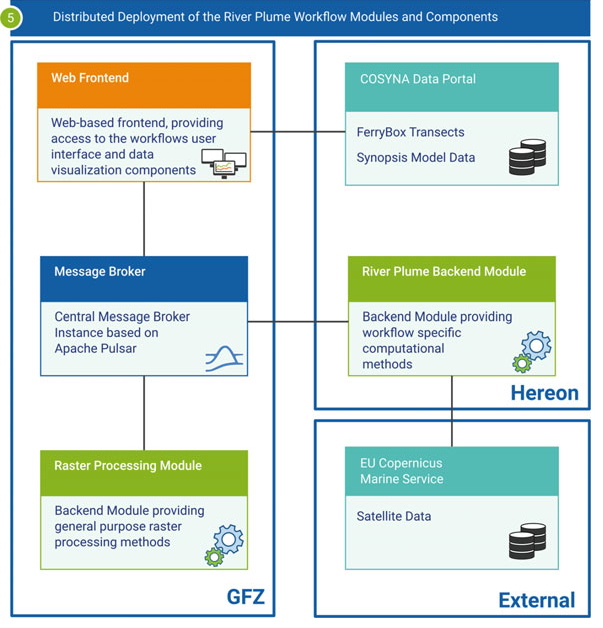
Fig. 15 Overview of the Riverplume Workflow’s modular implementation
The workflow’s modular structure is a design decision stemming from its beginnings as part of the Digital Earth project. It was necessary to develop modular code and enable the distribution of components across scientific centers to make the scientific workflow concept work for all involved fields, from terrestrial to marine geophysics applications. You can check out the results of this approach in the Flood Event Explorer (FEE).
The code for the River Plume Workflow is spread across three gitlab repositories:
The Frontend module contains the web-based frontend, including data visualization components.
The Synopsis Backend module contributes the data analysis methods specific to the River Plume Workflow, as well as methods for automatic data preprocessing.
Backend and frontend modules are connected through the DASF: Data Analytics Software Framework, which also allows to run the workflow on distributed IT-infrastructures.
Frontend module
The web user interface is based on django and vue.js.
Backend module
The de-synopsis-backend-module repository contains the River Plume Workflow’s analysis code in the RiPflow module, code needed for the MessageHandler, and routines for (automatic) data preprocessing. For more information, please check the README or the article in the How-To section of this manual. The RiPflow module contains all analyses that work with satellite data, such as anomaly detection, time series and looking up values for modelled waterbody positions.
Methods
This section is a collection of background information on the River Plume Workflow. It will take a step back from the implementation side and give context on some of the methods used in it.
The concept of scientific workflows
Since the Digital Earth project aimed to built bridges between different disciplines in Earth and Environment sciences, we used the concept of scientific workflows to break down complex scientifc questions into smaller, well-defined and re-usable components. For more details, please see Bouwer et al. 2022.
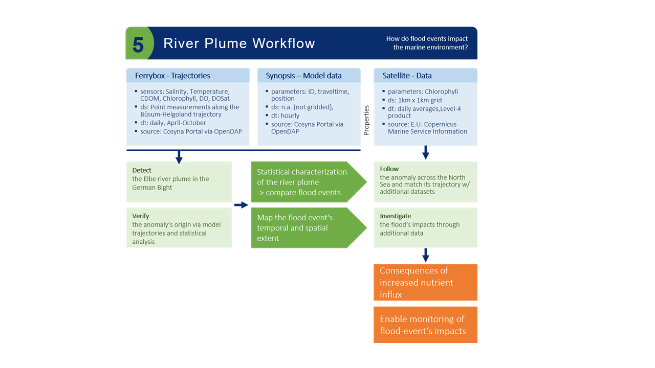
Fig. 16 Flowchart of the Riverplume Workflow
Fig. 16 shows the scientific workflow on which the Riverplume Workflow is based and the scientific questions that we were mainly interested in when we developed it, namely “How do riverine flood events impact the marine environment?”.
Ferrybox Data
The FerryBox data was retrieved through the Helmholtz Coastal Data Center Data Portal. Using the corresponding API, we were able to automatize the process of pre-processing the FerryBox data (see Task 4: Pre-process data for the Riverplume Workflow). For more information on the FerryBoxes, please refer to this article.
Synopsis Model Data & PELETS/2D
The drift model data was generated using the Lagrangian transport model PELETS/2D. Model data is currently only available for the summer of 2013.
Satellite data
We use satellite data from the Copernicus Monitoring Environment Marine Service (CMEMS), in particular North Atlantic Chlorophyll (Copernicus-GlobColour) from Satellite Observations: Daily Interpolated (Reprocessed from 1997) and Atlantic- European North West Shelf- Ocean Physics Reanalysis. The satellite information is used in the River Plume Workflow to estimate parameter values for the modelled water bodies’ positions, to generate time series along simulated trajectories and as an option for detecting anomalies automatically.
Automatic Data Processing Pipeline
As described in Task 4: Pre-process data for the Riverplume Workflow, new FerryBox data needs to be pre-processed before being used in the River Plume Workflow. We automated this process by setting up a cron daemon on our local cluster to search for new FerryBox data in the data base and, if available, pre-process it and upload it to a server, where the River Plume Workflow can access it. The script that automatically queries the HCDC data portal and pre-processes new data is available in the Synopsis Backend Module under DataGeneration/.
Anomaly Detection w/ Gaussian Regression
The automatic anomaly detection feature, that finds river plume candidates as anomalies in FerryBox data, is described in detail here: Bouwer et al. 2022, Ch.4.
Multiple linked views
How (and why) we used linked interactive components for the frontend can be found here: Bouwer et al. 2022, Ch. 3.
Contributions
The River Plume Workflow is one part of the Digital Earth Flood Event Explorer. It was developed in close cooperation between the Helmholtz centers Hereon and GFZ.
List of Contributors
Nicola Abraham
Holger Brix
Ulrich Callies
Daniel Eggert
Carlos Garcia Perez (HMGU)
Daniela Rabe
Philipp Sommer
Yoana Voynova
Viktoria Wichert
Your contributions
We invite you to contribute to the River Plume Workflow! If you are a user of the workflow, we are interested in your general feedback, how you use the workflow, and which additional functions you would be interested in. Please contact us via email or through the issue tracker in our gitlab repository.
References
Laurens M. Bouwer, Doris Dransch, Roland Ruhnke, Diana Rechid, Stephan Frickenhaus, and Jens Greinert, eds. 2022. Integrating Data Science and Earth Science: Challenges and Solutions. SpringerBriefs in Earth System Sciences. Cham: Springer International Publishing. https://doi.org/10.1007/978-3-030-99546-1
Daniel Eggert, and Doris Dransch. 2021. “DASF: A Data Analytics Software Framework for Distributed Environments.” https://doi.org/10.5880/GFZ.1.4.2021.004
Fabian Pedregosa, Gaël Varoquaux, Alexandre Gramfort, Vincent Michel, Bertrand Thirion, Olivier Grisel, Mathieu Blondel, et al. 2018. “Scikit-Learn: Machine Learning in Python.” http://arxiv.org/abs/1201.0490.
Daniela Rabe, Daniel Eggert, Viktoria Wichert, and Nicola Abraham. 2022. “The River Plume Workflow of the Flood Event Explorer: Detection and Impact Assessment of a River Plume.” https://doi.org/10.5880/GFZ.1.4.2022.006.
Viktoria Wichert, Daniela Rabe, Nicola Abraham, Holger Brix, and Daniel Eggert. 2022. “River Plume Workflow - Synopsis Backend Module.”
Ulrich Callies, Markus Kreus, Wilhelm Petersen, and Yoana G. Voynova, 2021. “On Using Lagrangian Drift Simulations to Aid Interpretation of in situ Monitoring Data” Frontiers in Marine Science https://www.frontiersin.org/articles/10.3389/fmars.2021.666653
Petersen, Wilhelm. 2014. “FerryBox Systems: State-of-the-Art in Europe and Future Development” Journal of Marine Systems. https://doi.org/10.1016/j.jmarsys.2014.07.003